The FIRE (Financial Independence, Retire Early) movement became popular in the 2010s, with much interest generated since then by early retirement and frugal blogs such as the Mr. Money Mustache blog (started 2011). The inspiration behind the FIRE movement is often attributed to the 1992 best-selling book Your Money or Your Life written by Vicki Robin and Joe Dominguez as well as the 2010 book Early Retirement Extreme by Jacob Lund Fisker.
Robin and Dominquez have sold more than a million copies of this book, inspiring readers with pithy wisdom such as . . .
"Money is something we choose to trade our life energy for.”
"The only real asset you have is your time. The hours of your life.”
"If you live for having it all, what you have is never enough.”
― Vicki Robin, Your Money or Your Life
The movement is mainly value driven as the quotations above suggest, but there's also much technical advice about the mechanics of how to achieve this financial independence and retire early. Much of this advice targets saving and tax efficiency strategies like Roth ladders, tax diversification, Roth conversions, and qualified and non-qualified account distribution advice. And of course there's plenty of criticism although recently the FIRE advocates have developed some overdue respect from FIRE skeptics in mainstream financial pages.
Someone trying to explore FIRE—financial independence, phased retirement options, and downsizing—will have a lot to think about. But the most critical and obvious problems are often lost in the technical weeds of tax efficiency strategies as if once you discover the secrets of a Roth ladder things will begin to fall into place.
Tax efficiency is mere fine tuning in comparison to the larger, glaring problem of cash flow, or what economists call, consumption smoothing.
One of the reasons this critical issue of cash flow (the search for smooth annual spending allowance) is not often addressed is that its difficult to observe and nearly impossible to solve for in conventional planning software. Conventional planning software varies of course in its features, sophistication, details, and reporting, but one thing all conventional software programs have in common is that they all begin with the question—indeed, nearly the first data point they ask for—"how much do you need to live on in retirement?"
Thus, from the get go, the prevailing assumption is often that there has to be two levels of living standard: pre- and post-retirement. There is no standard approach, but it's common to read that financial independence involves a severe belt tightening in the near term in order to breath easier in some future years, especially when early retirement is the goal. But most importantly, note that the annual spending is determined by the user or the planner, not discovered by the planning software. This is important and it changes everything. This old approach is driven by the limitation of conventional planning tools not because it's the best approach.
The following case study illustrates how a different approach can help solve these puzzles. Instead of assuming that the user must stipulate his or her spending level needs (supply an exogenous data variable), MaxiFi Planner allows users to explore financial plans that internally calculate or discover the native or endogenous annual spending levels. When we are no longer constrained by the need to supply the annual spending target as a guess or a hope and can instead let the program discover the annual spending target, we have a whole new way to approach the lifetime planning puzzle and evaluate the possibilities of FIRE, financial independence and the hope of early retirement.
I will illustrate these principles with an admittedly stereotypical enthusiastic FIRE financial planner couple. The aim here is not to represent this couple with any kind of claim this approach works the same in every case, for no two household economies are alike. If the details listed directly below don't represent you, the reader, or what you imagine a typical family in this situation might look like, remember, the point is really about the methodology and approach to things discovered, not the details themselves.
Here are the broad parameters of the case:
- The 32-year old couple, together, have $230,000 in annual labor income.
- Their fixed spending comprises housing, retirement contributions, and taxes. Later in life it includes Medicare B premiums.
- The family has accumulated $400,000.
- The family owns a $200,000 home with 15 years left on the mortgage
- Where early or phased retirement begins, $15,000 annually is added for high deductible health insurance.
- Where "early" retirement begins in these scenarios, labor earnings (along with corresponding employer contributions to retirement) drop after 2030 from $230,000 to $50,000 of household income.
Again, the effort here is to illustrate MaxiFI's approach to evaluating the impact of early or severely reduced employment earnings beginning at age 42 for this 32-year old couple.
The game we will play with this hypothetical family involves first lowering their annual salary from a combined $230,000 annual income to a combined annual income of $50,000 beginning at age 42 through age 60. During that 18-year period of freelance income, I have added an additional $15,000 of annual insurance costs. I will experiment with two variables in particular that we have control over in building the lifetime plan: we can control when Social Security begins (taking advantage of delayed retirement credits) and I will experiment with when to start and end the withdraw of retirement assets. These are just two of a number of variables we could change. For example, a user exploring FIRE options could also experiment with the following variables:
- Roth conversions or building Roth ladders
- downsizing a home
- buying a tiny home and travel for 5 years, lowering housing costs
- moving to a more tax-friendly state
- working longer or shorter
- extending the freelance period of earnings past the age of 60
- paying down a mortgage more quickly or refinancing to change the cash flow
- changing the retirement withdraw start dates or end dates or both
Again, the main point here is to illustrate through the use of just two of these many available variables that we can change the level of annual spending as well as the shape or trajectory of this annual spending over the life of the plan. Creating a viable plan is the first order of business and only after that can we begin to use clever tax advantage strategies to shave a bit more off of taxes and thus raise spending levels.
Stay Fully Employed
This first chart below can serve as a benchmark we will return to at the end of our analysis. It represents the available annual spending if the couple remain fully employed through age 60. The chart shows the green line, annual income, highlighting three periods in life beginning with labor earnings, then a period where there's only retirement withdraws, and finally a third period where there's retirement withdraws and Social Security income. But this is income, and it is smooth spending we want, not smooth income. The blue line shows fixed spending comprising housing, taxes, contributions to retirement, and late in life, rising Medicare B premiums. And most importantly, the orange line, the internally calculated annual discretionary spending. This is the safe, annual spending allowance. It might also be referred to as household living standard. It represents what there is to live on after or net of fixed spending. All charts are in today's dollars and thus account for inflation.
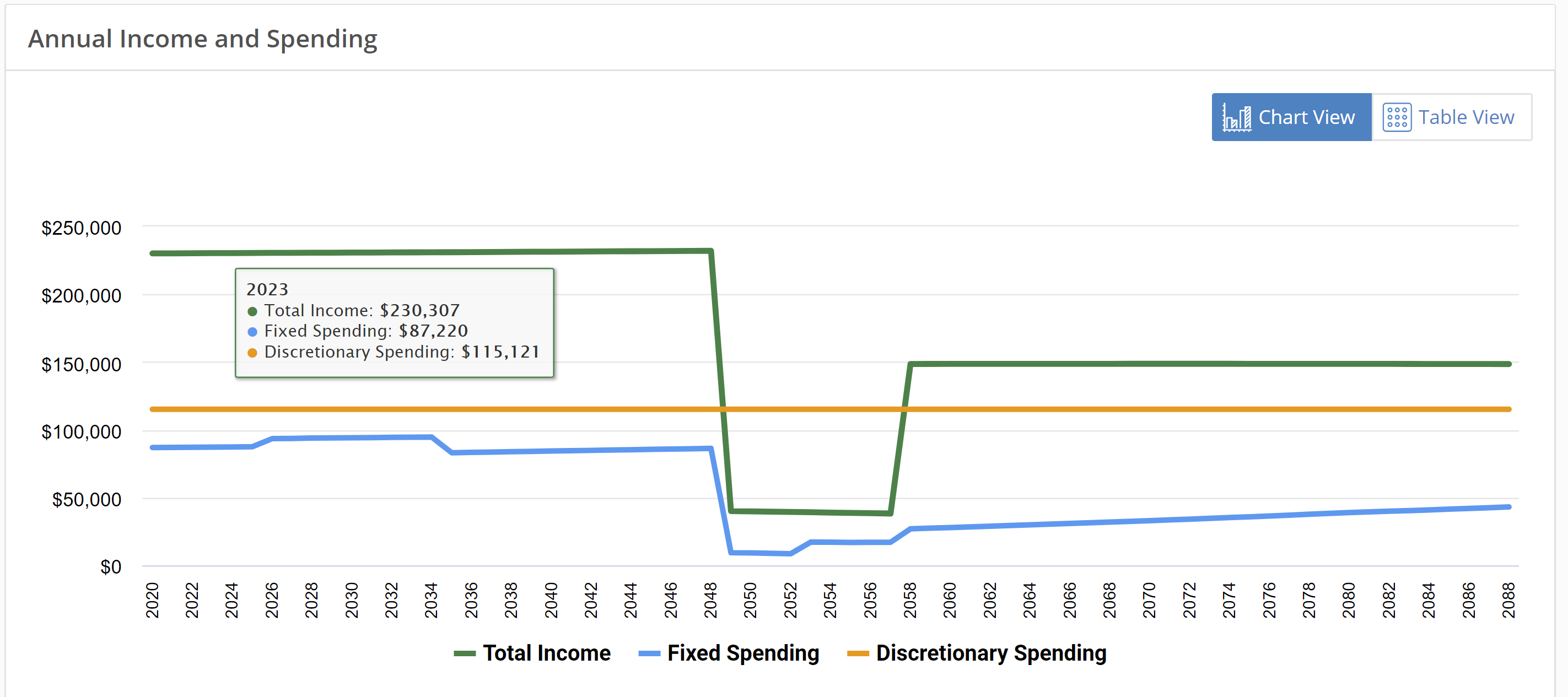
The discretionary spending is the primary concern in this analysis because it represents what the couple has to live on after paying fixed expenses. It's important to emphasize that this is an internally calculated, native, or "endogenous" spending level. It's not what the user needs or hopes for or even wants. It's what is mathematically available given the constraints and resources in the model. The amount represented by the orange line as well as the shape of that line is the "answer" to the question: Can we retire early?
Users unfamiliar with financial planning software may not appreciate this upside down approach that solves to find your native available annual spending level. For in nearly every, if not all, conventional planning programs the user enters this annual amount. From the MaxiFi point of view, this user interference involves trying to do the work of the software for it, and doing it very poorly because it is basically guesswork. Furthermore a manual entry by the user—because it is user-entered instead of native to the calculation—does not change dynamically with each variation in the plan. Once you manually enter a spending level using the conventional approach, you are stuck with it and it won't change until you change it to something else. So if you enter that you spend, say $60,000 per year, that number would not change if you told your model that you wanted to downsize your home, postpone Social Security, or even take on an extra job or move to part time work. But with MaxiFi, even the slightest change in the model—imagine a $200 one-time fixed expense entered to appear 37 years from now—will change your lifetime spending levels and show up as differences in annual spending levels, even if trivially so.
This ability to chart native or endogenous spending levels with every change in the plan is a game changer for FIRE users because the consequences of working more or less, phasing out or retiring sooner or later, living in a tiny house or a sailboat for 10 years can be understood in terms of the annual change in available discretionary spending allowed rather than some highly abstract percentage chance of not running out of money at the end of life as we'd see in conventional planning.
So lets look at this same chart from above one more time and call attention to the orange line. The orange line below is the internally calculated annual discretionary spending. In this case it is $115,121. This is the safe, annual spending allowance the household will have if they continue working full time through age 60. It could also be referred to as household living standard. It represents what there is to live on net of fixed spending. It also represents what the household will be giving up as they explore these retire early options.
The Retire Early Options
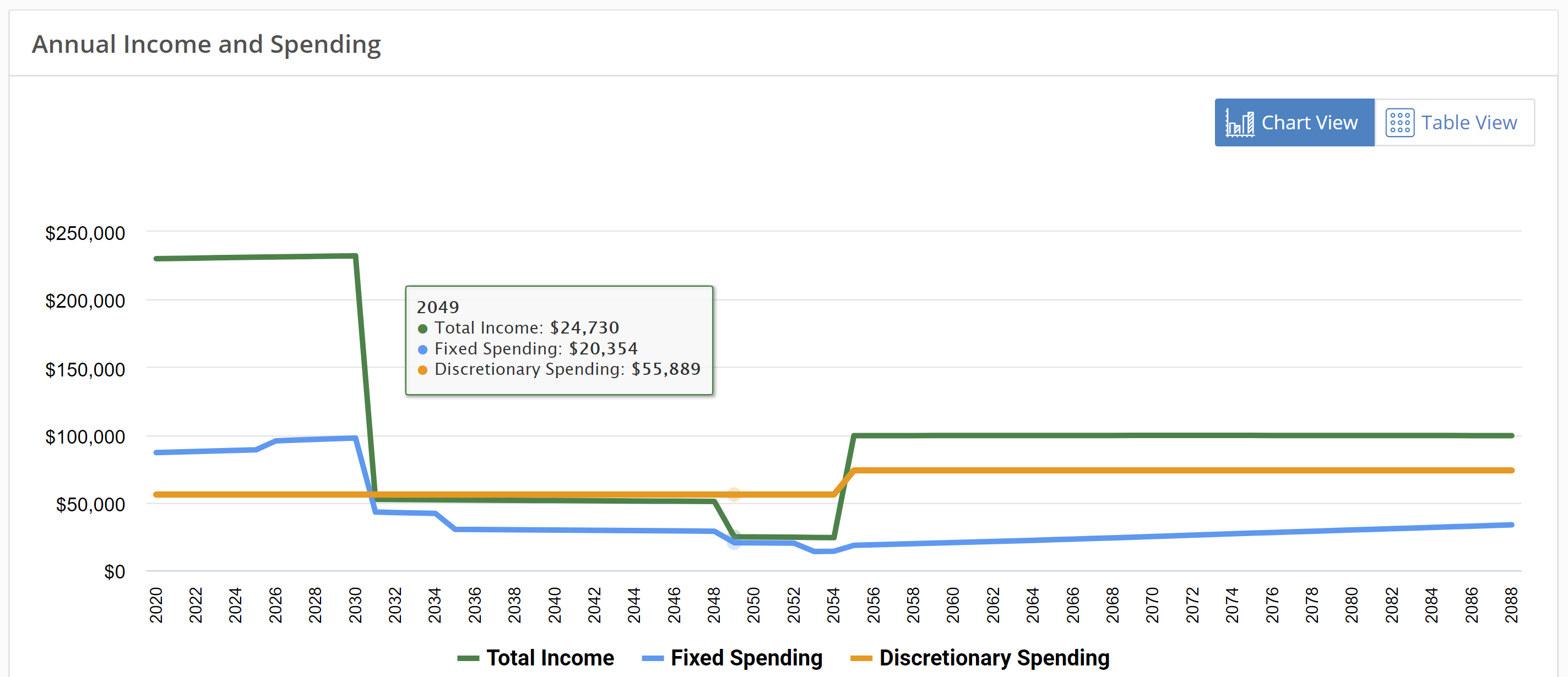
In the next variation of this plan, you can see below that total income has dropped off quickly at age 42 to the new freelancer, phased retirement level of $50,000 annual income. The fixed spending has a fairly similar pattern to the chart above as one would expect, but discretionary spending has dropped considerably. Discretionary spending is now at $55,899 until Social Security kicks in at age 67. Remember, it's annual spending level, not income, that we are concerned about.
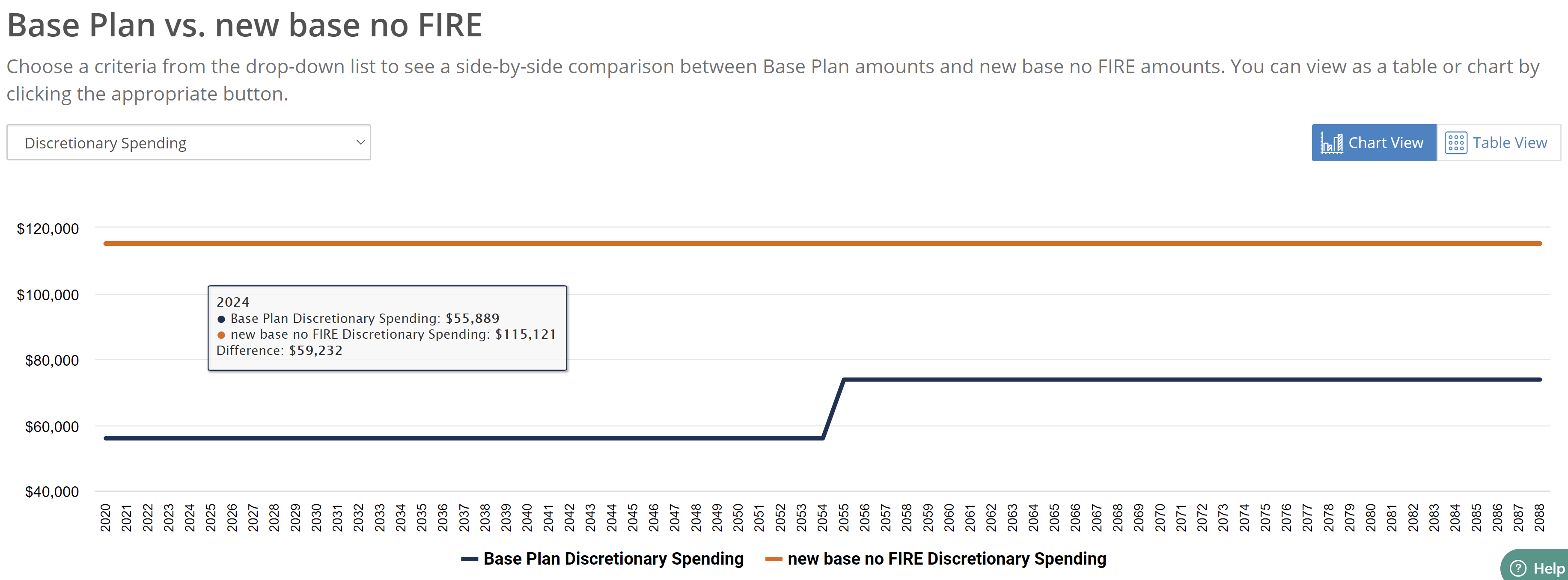
Below, the discretionary spending levels for the two models above are compared and going forward I will refer to the retire early model as our "base plan."
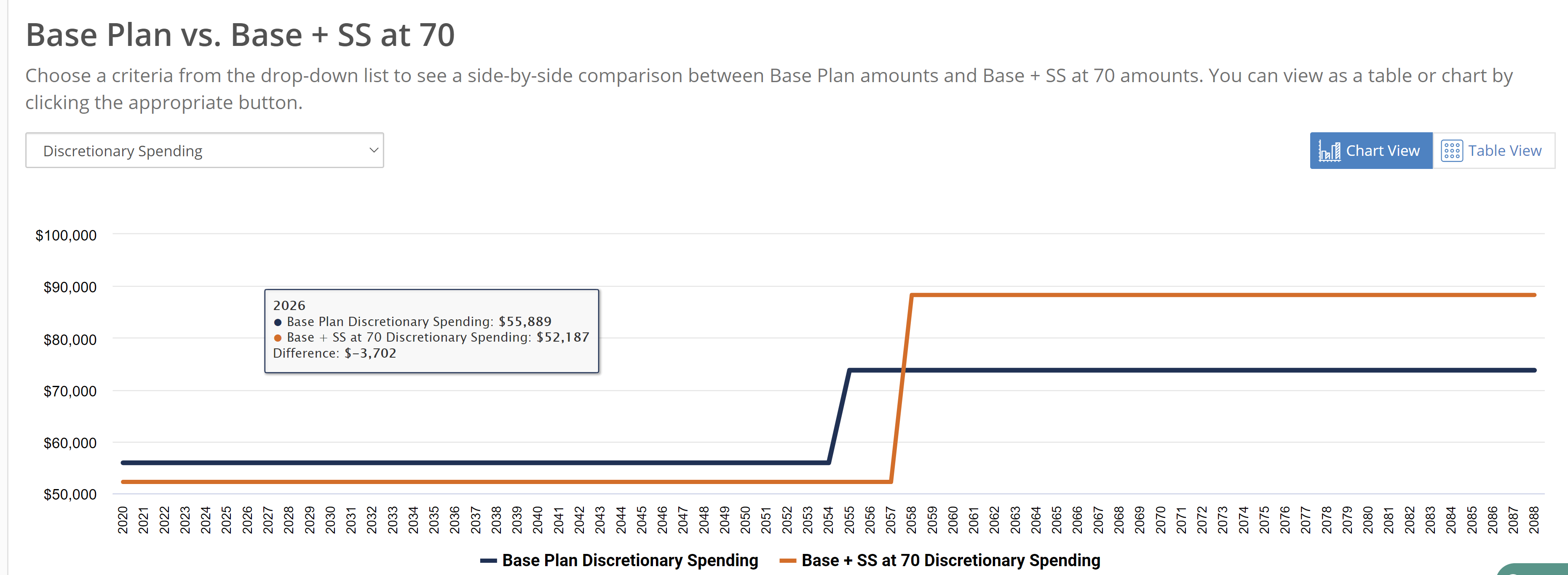
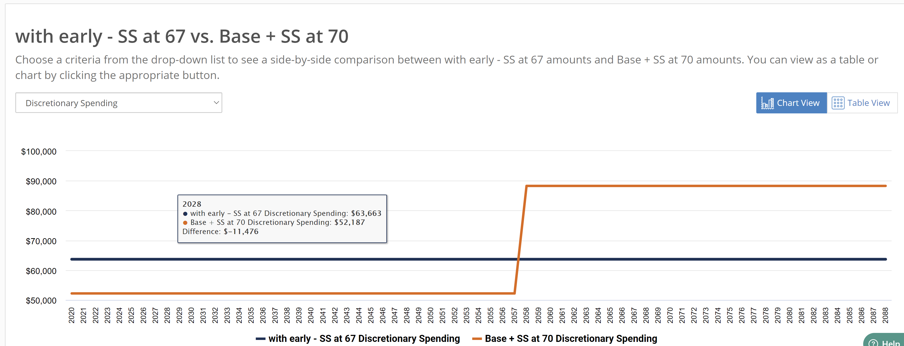
The next version of this plan will consider the impact of postponing Social Security to age 70 and taking delayed retirement credits. Below, the retire-early base plan with Social Security at age 67 is compared to the same plan but with Social Security set to begin at age 70. The impact of this change makes worse the liquidity constraint or cash constraint (notice the lower spending in the near term and higher in the far term) as you see represented by the orange line below. But over the life of the model it does raise the present value of lifetime spending, but because of the constraint, it may not be as practical as taking Social Security age 67.
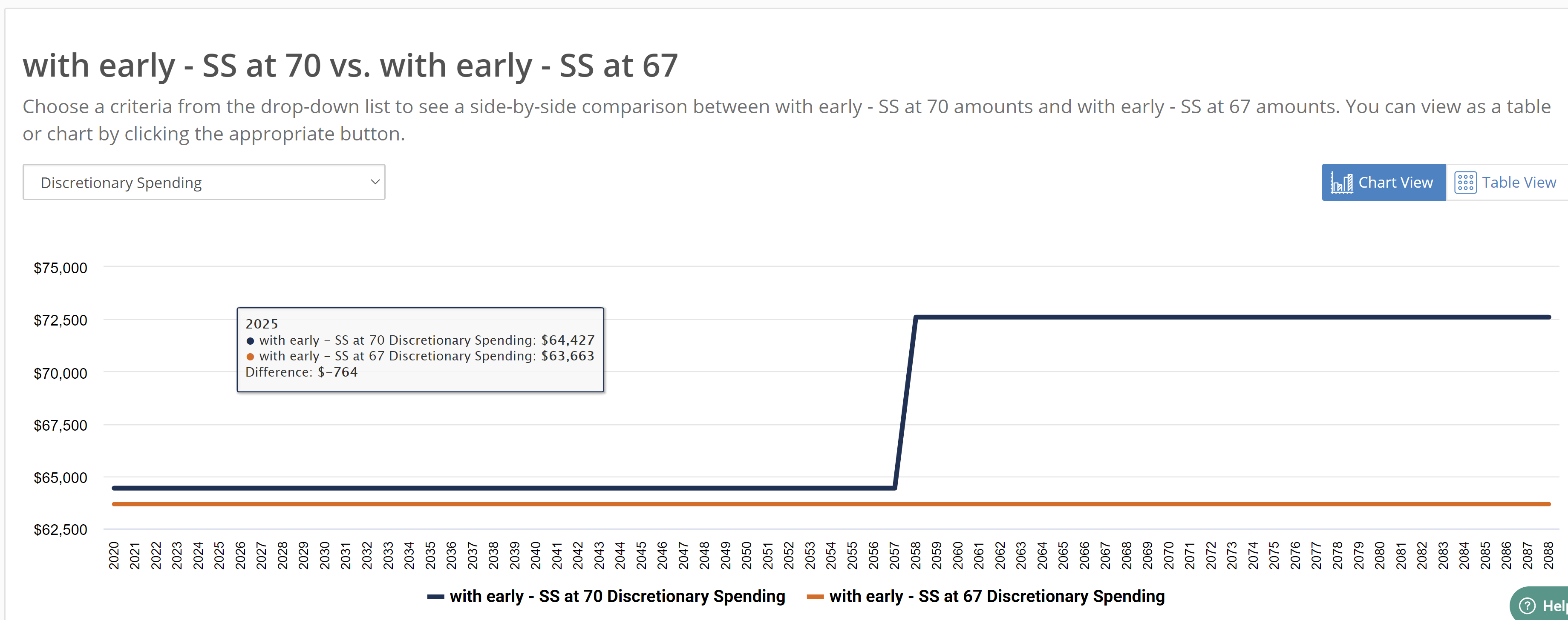
To address this liquidity constraint, in the next variation I will put Social Security back to age 67 and change the dates of the retirement withdraws in an attempt to raise the near term spending levels. The orange line below represents the withdraw dates unchanged and Social Security at 70 (just like above) but with retirement withdraws beginning at age 61 and ending at 100 compared to the blue line where Social Security age is at 67 but the retirement withdraws begin at age 61 and end at age 70. The annual spending allowance that is a result, the blue line, is now flat. Again, this was accomplished by taking all of the retirement account withdraws between age 61 and 70.
In the chart below, the Social Security start date is set back to age 70 and the retirement withdraw dates of 61-70 used as in the chart above. Now, in this alternative, the blue spending allowance line is higher than the orange line both in the near term and the far term. We are discovering that the safe, annual spending allowance is changing automatically when we change key variables in the model. The plan is not stuck with the static user's input: "I need $60,000 to live on in retirement." Instead, a new available annual safe spending is revealed with each change in variables or assumptions in our plan.
Finally, the chart below compares the best FIRE option discovered —the blue line—with the starting option of continuing to work full time through age 60, the orange line.
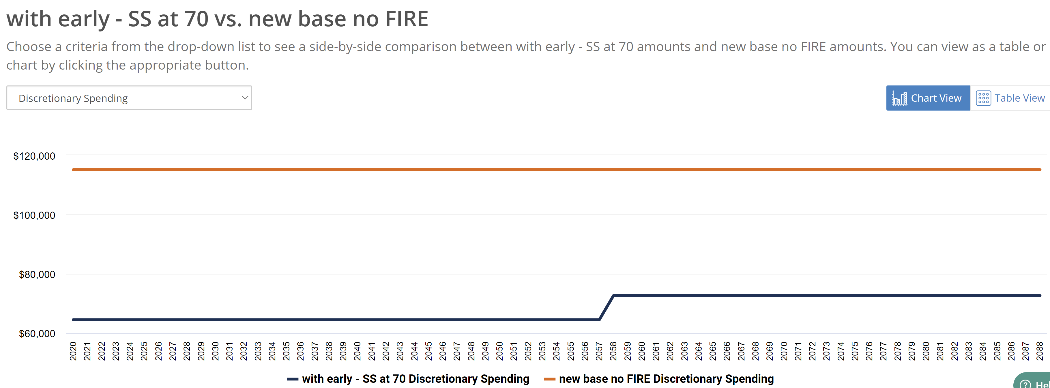
Realizing that a planning program can calculate available annual spending and provide the levers to change the shape of this annual spending allowance line is an extremely important discovery and a radically different approach compared to working piecemeal with tax saving strategies and implementing such strategies blind to their impact on annual spending. Furthermore, the larger patterns of cash flow or annual spending are found to be far more critical to the decision making process of a FIRE proponent than the smaller details of tax saving in one set of years or another. Of course a plan can be fine tuned to take advantage of tax efficiencies that might be discovered in a Roth conversion or a Roth ladder, but the first order of business is to discover an annual spending allowance by moving these macro levers as described above.